Classification with sparklyr

In this post I will use fairly new R package sparklyr which allows you to connect from Spark with R to use Spark’s machine learning library. All with a complete dplyr backend. To connect to a local instance of Spark, you first need to spark_install and then connect to that instance with spark_connect where the master argument should be “local”

I will use the flights data from nycflights13 package to try to predict flights that will be delayed. As I import the data, I also create a new weekday variable

library(sparklyr)
library(dplyr)
sc <- spark_connect(master = "local", version="2.1.0")

flights_data <- nycflights13::flights %>% 
  mutate(weekday=weekdays(as.Date(paste0(year,"-",month,"-",day))))

To upload this data frame into my local instance, use copy_to()

flights_sdf <- copy_to(dest = sc, df = flights_data, name = "name", overwrite=T)

Then, I create a new variable i) Delay is 1 if the plane was delayed, ii) Car is 1 if the flights is flown by one of the four selected carreirs, iii) Night that is 1 if the the departure was after 6 pm or earlier than 6am and iv) Weekendif the departure was on a Sunday.

flights_sdf = flights_sdf %>% 
  mutate(Delay = if_else(dep_delay>0,1,0)) %>%                           # (i)
  mutate(Car = if_else(carrier %in% c("DL","US","DH","UA"),1,0)) %>%     # (ii)
  mutate(Night = if_else(hour>=18 | hour<=6,1,0)) %>%                    # (iii)
  mutate(Weekend = if_else(weekday=="Sunday",1,0))                       # (iv)

I create a new data frame logit_sdf with the constructed variables, and exluce all missing values

logit_sdf = flights_sdf %>% 
  mutate(DepHour = hour) %>% 
  select(Delay, Car, Night, Weekend, DepHour) %>% 
  na.omit()

## * Dropped 8255 rows with 'na.omit' (336776 => 328521)

I divide the dataset into two parts, one for training and one for testing, and then fit the binary logistic regression model with the Spark Machine Learning function ml_logistic_regression

partitions <- sdf_partition(logit_sdf, training=0.7, test=0.3, seed=6789)
trainset <- partitions$training
testset <- partitions$test
ml_model <- trainset %>% ml_logistic_regression(formula = Delay ~ DepHour + Car + Night + Weekend)
summary(ml_model)

## Call: ml_logistic_regression.tbl_spark(., formula = Delay ~ DepHour + Car + Night + Weekend)  
## 
## Coefficients:
## (Intercept)     DepHour         Car       Night     Weekend 
## -1.88682995  0.11464268 -0.06620449 -0.19125631 -0.08851651

Prediction is done with sdf_predict. Also a matrix with TP = True positive, FP = False positive, TN = True negative, FN = False negative. For now, I consider the cut-off value for when we would classify a predicted probability as a delay to be 0.5. The model falsely predict roughly 29 thousand flights as delayed when they were in fact not.

predvals <- sdf_predict(x = testset,model = ml_model)      


score_test <- predvals %>% 
  mutate(Event = if_else(probability_1_0 >= 0.5,1,0)) %>%   
  mutate(TP = if_else(Event==1 & Delay==1, 1, 0)) %>%       
  mutate(FP = if_else(Event==1 & Delay==0, 1, 0)) %>%       
  mutate(FN = if_else(Event==0 & Delay==1, 1, 0)) %>%       
  mutate(TN = if_else(Event==0 & Delay==0, 1, 0))%>%        
  summarise(nTP = sum(TP, na.rm=T),
            nFP = sum(FP, na.rm=T),
            nFN = sum(FN, na.rm=T),
            nTN = sum(TN, na.rm=T)) %>%                     
  select(nTP,nFP,nFN,nTN)                                   

mat <- t(matrix(score_test %>% collect(),ncol=2,byrow=T,dimnames=list(
  c("TRUE", "FALSE"),
  c("Predicted: TRUE", "Predicted: FALSE")
)))

mat

##                  TRUE FALSE
## Predicted: TRUE  9640 28893
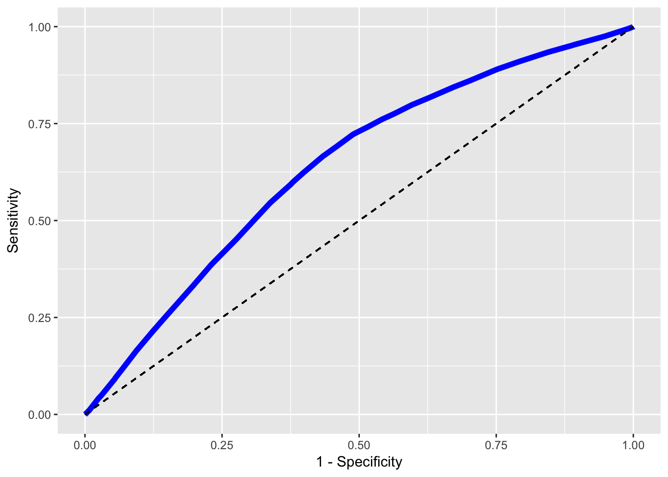
## Predicted: FALSE 8734 51136

Instead of using a specific cut-off value as above, it is better to look at a ROC-curve. Here I use the previous code to construct a function calc_roc that will output the sensitivity and specificity of the model given a specified cut-off value. I will then loop through a sequence of different cut-off values and see how sensitivity and specificity changes for different cut-off values. A much more rigorous method of evaluating the model.

calc_roc <- function(x, k=0.5){                               
 
  x <- x %>% 
    mutate(Event = if_else(probability_1_0 >= k, 1, 0)) %>%  
    mutate(TP = if_else(Event == 1 & Delay==1, 1, 0)) %>%     
    mutate(TN = if_else(Event == 0 & Delay==0, 1, 0)) %>%     
    mutate(P = if_else(Delay == 1, 1, 0 )) %>%                
    mutate(N = if_else(Delay == 0, 1, 0)) %>%                 
    summarise(n1 = sum(TP, na.rm = T),
              n2 = sum(P, na.rm = T),
              n3 = sum(TN, na.rm = T),
              n4 = sum(N, na.rm = T)) %>%                    
    summarise(val1 = n1/n2,
              val2 = n3/n4) %>%                              
    
    select(Sensitivity = val1, Specificity = val2)
  
  return(x)                                                
  }


pred <- predvals %>% collect
perf<-vector()  

for(i in seq(0,1,by=0.01)){
  perf <- rbind(perf, do.call(calc_roc, list(pred,i)))
}

colnames(perf) <- c("Sensitivity","Specificity")

The result can then be plotted using ggplot2.

library(ggplot2)
ggplot(perf, aes(x=1-Specificity, y=Sensitivity))+
  geom_line(col="blue",lwd=2)+
  geom_segment(aes(x=0,xend=1,y=0,yend=1),linetype=2)

erst

Classification with sparklyr